Icona progetto

Road Sign Detection

using YOLO

Problem

In our project, we present a supervised method of detecting traffic-signs completely based on deep Convolutional Neural Networks (CNNs). We will use Darknet, an open source neural network framework, and Google Colaboratory, a free environment that runs entirely in the cloud and provides a GPU.

Motivation

Traffic-sign recognition (TSR) is a technology by which a vehicle is able to recognize the traffic signs put on the road e.g. "Give Way" or "Obligation Straight-Turn Right" or "Pedestrian Path". This is part of the features collectively called ADAS. The technology is being developed by a variety of automotive suppliers. It uses image processing techniques to detect traffic signs. The detection methods can be generally divided into color-based, shape-based and learning-based methods.

In this regard we have thought of an urban scenery on which we have placed some signals and a traffic light in a rather random order. First of all, a 3D model of the circuit was created with the 3ds max, followed by renderings in various perspectives, and one containing all the measurements of the circuit.

For 3D models click here: 3D Model

Subsequently, the circuit was made on the basis of the 3D model. Colored cards and ribbons were used. for the construction of the roads, while the signs are made of wood. In addition, brown cardboard boxes were used to isolate the circuit from the surrounding scenery. Below are pictures of the result:

Goals

Main objectives

  1. Creating the Dataset
  2. Train a Convolutional Neural Network
  3. Improve Object Detection

Method

Creating the Dataset

In this phase, the dataset was generated starting from the sampling of the single signals placed in the foreground and captured according to different perspectives. (an example is shown below)

The tool used to label classes is LabelImg:

LabelImg generates for each image a file marked Yolo, for example image1.jpg will have the corresponding image1.txt in the same folder.

The .txt file has this type of format (see RED box):

It has coordinates in Yolo format object-id, center_x, center_y, width, height.

- object-id represents the number corresponding to the category of objects that i listed in the 'classes.txt' file,

- center_x e center_y represent the central point of the selection rectangle,

- width e height represent the width and height of the rectangle,

After reaching an exhaustive number of instances per class, it was possible to proceed to the Object Detection phase.


Object Detection

The algorithm used for object detection is YOLO (You Only Look Once) which uses Daknet, an open source neural network framework written in C and CUDA that supports CPU and GPU computation.

The CNN divides an image into regions and then it predicts the boundary boxes and probabilities for each region. It simultaneously predicts multiple bounding boxes and probabilities for those classes.

YOLO sees the entire image during training and test time so it implicitly encodes contextual information about classes as well as their appearance.

With the help of the Anchor Boxes, the algorithm is able to recognize multiple objects within a single cell, they are extrapolated directly from the training set by clustering the Bounding Boxes using K-means algorithm.

It is also able to make predictions on 3 different scales, reducing the image in order to increase accuracy

At the end of the processing, the bounding boxes with the highest confidence are kept, discarding the others.

The following project uses YOLO 4 version.

In experiments, YOLOv4 obtained an AP value of 43.5 percent (65.7 percent AP50) on the MS COCO dataset, and achieved a real-time speed of ∼65 FPS on the Tesla V100, beating the fastest and most accurate detectors in terms of both speed and accuracy. YOLOv4 is twice as fast as EfficientDet with comparable performance. In addition, compared with YOLOv3, the AP and FPS have increased by 10 percent and 12 percent, respectively.

Implementation and Code

After loading the project folder on the drive, we have created a new Google Colaboratory session for training the neural network.

  • in Colaboratory file, need to change the runtime type: from Runtime menu select Change runtime type and choose GPU as Hardware accelerator.

Configuration

In this section we will proceed to configure our Darknet network.

We will proceed to mount Google Drive on the Colab session

from google.colab import drive
print("mounting DRIVE...")
drive.mount('/content/gdrive')
!ln -s /content/gdrive/My\ Drive/root_folder/my_drive

Now we will proceed to clone the repository , we're going to set some configuration parameters such as:
- OPENCV to build with OpenCV;
- GPU to build with CUDA to accelerate by using GPU;
- CUDNN to build with cuDNN v5-v7 to accelerate training by using GPU;
- CUDNN_HALF to speedup Detection 3x, Training 2x;

The next step is the compile.

!git clone https://github.com/AlexeyAB/darknet
%cd darknet
print("activating OPENCV...")
!sed -i 's/OPENCV=0/OPENCV=1/' Makefile

print("engines CUDA...")
!/usr/local/cuda/bin/nvcc --version

print("activating GPU...")
!sed -i 's/GPU=0/GPU=1/' Makefile

print("activating CUDNN...")
!sed -i 's/CUDNN=0/CUDNN=1/' Makefile

print("activating CUDNN_HALF...")
!sed -i 's/CUDNN_HALF=0/CUDNN_HALF=1/' Makefile

print("making...")
!make

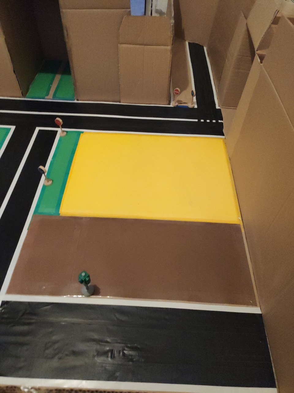
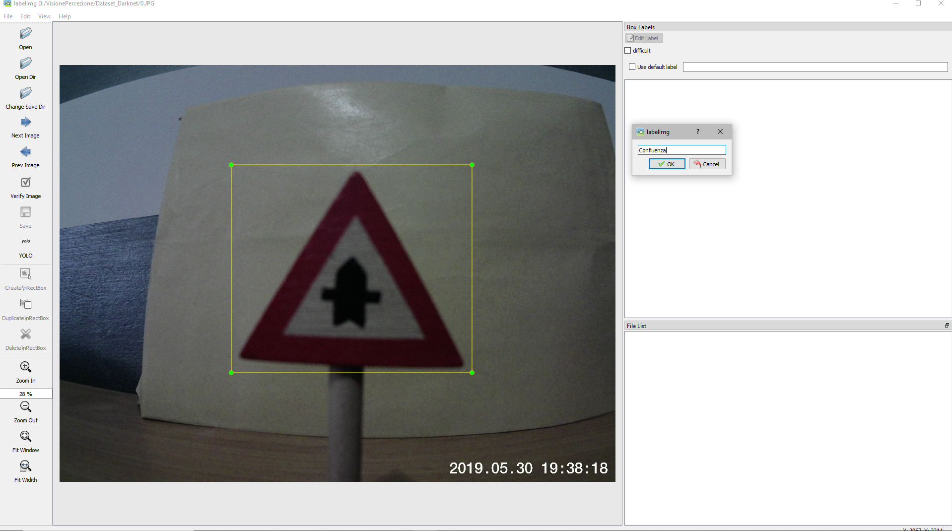
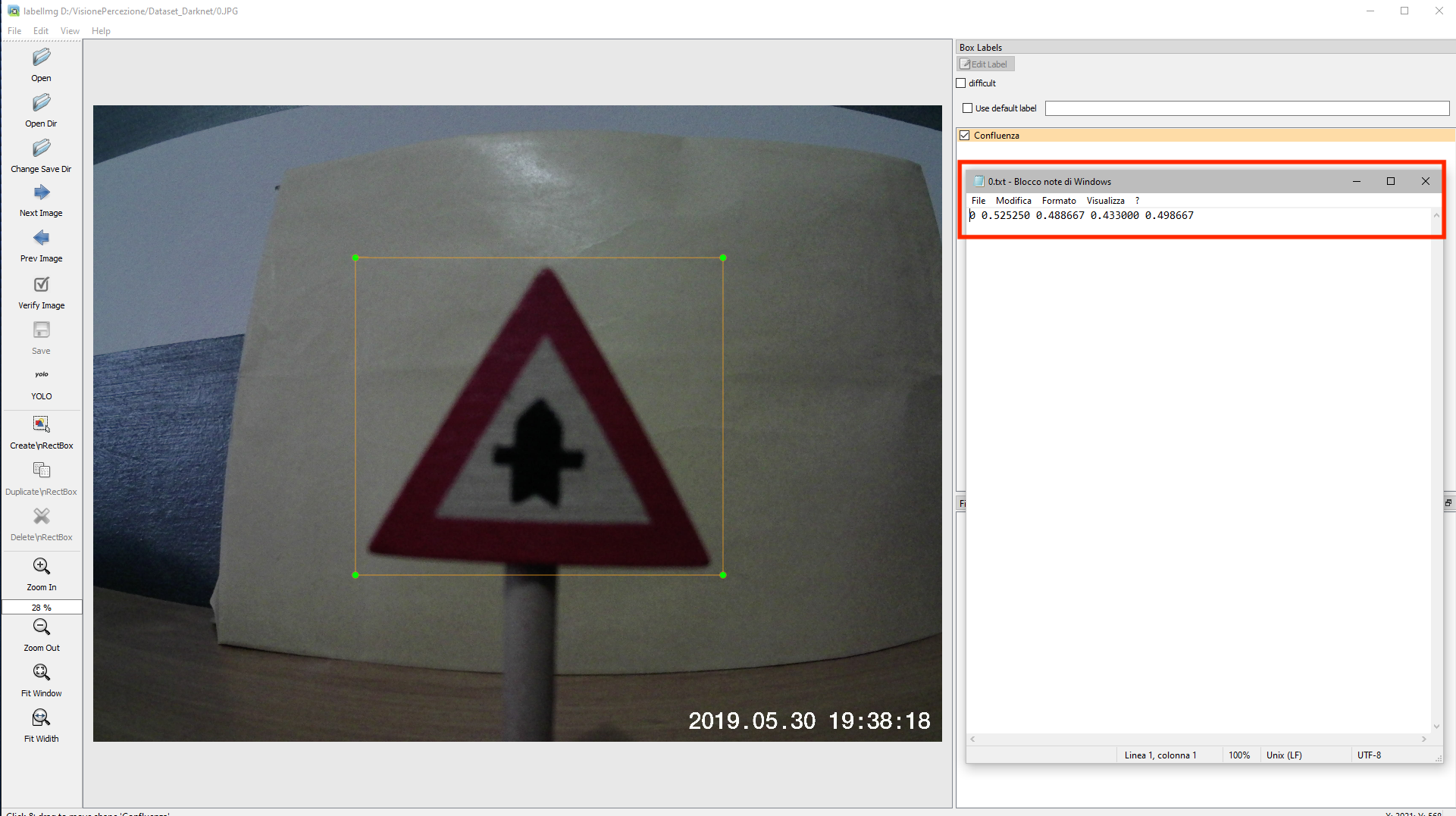
To proceed we will load the dataset in order to use it for training.

The idea is to insert in a folder called obj all the images .jpg with the relative files.txt and then compress the folder.

print("loading dataset...)
!cp /my_drive/dataset_folder/obj.zip ../

And now we can unzip it.

print("unziping dataset...")
!unzip ../obj.zip -d data/obj.zip ../

It is important to also load the main yolo-obj.cfg configuration file, which will contain information for the construction of the network, such as the size of the images, the number of classes, filters, any augmentation techniques and more.

The file is located in the folder configuration_files.

The main changes that have been made are shown below:

  1. change line batch to batch=64
  2. change line subdivisions to subdivisions=16
  3. change line max_batches to (classes*2000 but not less than number of training images, but not less than number of training images and not less than 6000): max_batches=28000
  4. change line steps to 80% and 90% of max_batches: steps=22400,25200
  5. set network size width=416 height=416 or any value multiple of 32:
  6. change line classes=14 to your number of objects in each of 3 [yolo]-layers:
  7. change filters=57 to filters=(classes + 5)x3 in the 3 [convolutional] before each [yolo] layer, keep in mind that it only has to be the last [convolutional] before each of the [yolo] layers.

Darknet needs two more files:
- obj.names, which contains the name of the classes.

The file must be similar to the one generated during the dataset preparation phase. So it is important to respect the order of the classes..

class 0
class 1
class 2
class 3
class 4
...

- obj.data, which contain information about training and number of classes.

classes = number of classes
train = path_to/train.txt
valid = path_to/valid.txt
names = path_to/obj.names
backup = path_to/backup_folder

For loading configuration files:

print("loading yolo-obj.cfg...")
!cp /my_drive/configuration_files/yolo-obj.cfg ./cfg
print("loading yolo-obj.names..")
!cp /my_drive/configuration_files/yolo-obj.names ./data
print("loading yolo-obj.data..")
!cp /my_drive/configuration_files/yolo-obj.data ./data

Darknet needs a .txt files for training which contains filenames of all images, each filename in new line, with path relative, for example containing:

data/obj/img1.jpg
data/obj/img2.jpg
data/obj/img3.jpg
...

Specifically, we decided to split the dataset in:

  • 80% training set
  • 10% validation set
  • 10% test set

We have defined a Python script that does it: generate_train.py

Then, 3 .txt files are generated and saved on the Drive in the dataset_preparation folder:

  • train.txt
  • valid.txt
  • test.txt

Darknet offers the possibility to stop training at one point and resume it at a second moment:

  • if you start the training for the first time you need to save the txt files on the Drive in the specified folder.
  • if training is resumed from the point of interruption, the previously saved files must be loaded (to keep the dataset split unaltered)

START TRAINING FROM BEGINNING:

print("loading script...")
!cp /my_drive/py_scripts/generate_train.py ./
print("performing script..")
!python generate_train.py
print("copying .txt in Drive..")
!cp ./data/train.txt /my_drive/dataset_preparation/
!cp ./data/test.txt /my_drive/dataset_preparation/
!cp ./data/valid.txt /my_drive/dataset_preparation/

RESUME TRAINING:

print("loading train.txt...")
!cp /my_drive/dataset_preparation/train.txt ./data
print("loading test.txt...")
!cp /my_drive/dataset_preparation/test.txt ./data
print("loading valid.txt...")
!cp /my_drive/dataset_preparation/valid.txt ./data

For training, you need to download the pre trained weights (yolov4.conv.137) are used to speed up the workout. The approach is to use pre-trained layers to build a different network which may have similarities in the first layers.

This file must be uploaded to the backup folder

print("loading pre_trained weights...")
!cp /my_drive/backup/yolov4.conv.137 ./

Once the configuration phase is complete, it is possible to lead to the training phase

Training

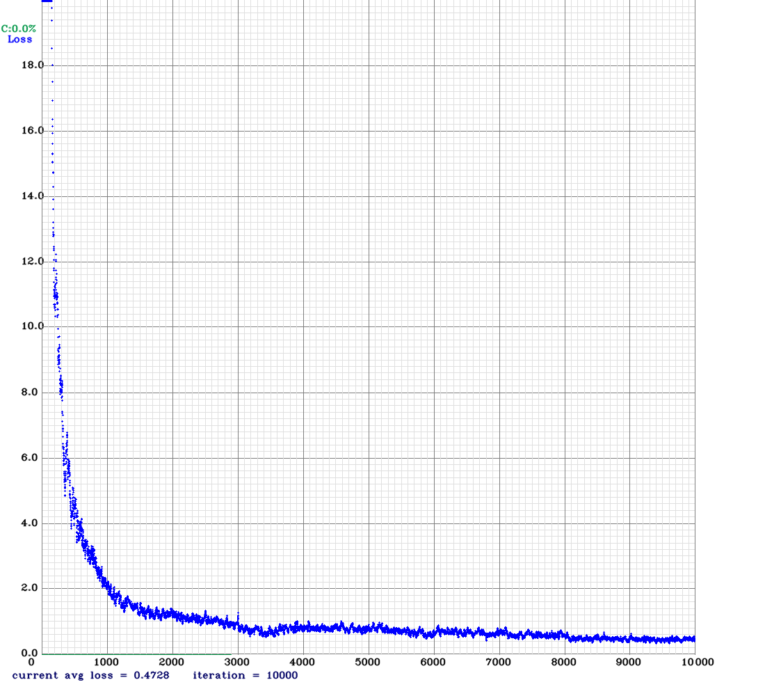
In this section, we will start training the network using the command line:

!./darknet detector train data/obj.data cfg/yolo-obj.cfg yolov4.conv.137 -dont_show

  • file yolo-obj_last.weights will be saved to the backup folder for each 100 iterations
  • file yolo-obj_xxxx.weights will be saved to the backup folder for each 1000 iterations

It is also possible to stop the training at a point (for example after 2000 iterations) and start again later from it:

!./darknet detector train data/obj.data cfg/yolo-obj.cfg /my_drive/backup/yolo-obj_last.weights -dont_show
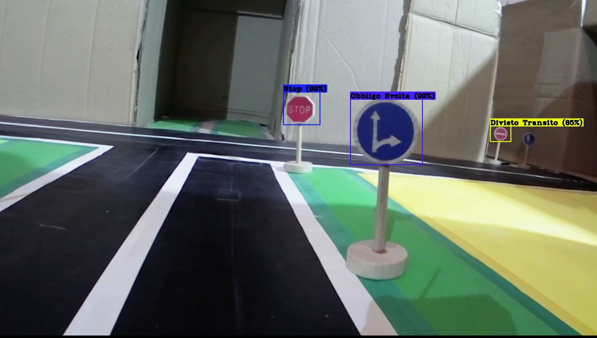
Detection

When the training is complete, we will perform object detection on the videos and save the results on the Drive.

  • increase network-resolution by set in your .cfg-file height=608 and width=608
  • change in obj.data file, from valid = path_to/valid.txt to valid = path_to/test.txt

Run the following command lines:

print("detecting...")
!./darknet detector demo data/obj.data cfg/yolo-obj.cfg /my_drive/backup/yolo-obj_xxxx.weights -dont_show /my_drive/test_videos/name_video -thresh .7 -i 0 -out_filename prediction.avi
print("save prediction in Drive...")
!cp prediction.avi /my_drive/predictions/name_prediction

For the resources Drive of the whole project: Google Drive

For all Python code on Github: YOLODarknet_code.ipynb

Dataset

The dataset consists of approximately 4780 images and 4780 corresponding .txt files.

Class n° Images
Intersection 260
Give Way 270
Right of Way 260
No Thoroughfare 280
No Overtaking 270
No Entry 270
Obligation Straight-Turn Right 300
Car Park 540
Pedestrian Path 290
Stop 290
Crosswalk 330
Green Light 530
Yellow Light 320
Red Light 570

Results

Qualitative Results

The video was made by placing a webcam on a hand-guided machine and tested for our neural network.

The following result shows the detection performed using 8000 weight as a model.

As can be seen, two detection errors are committed which occur mainly on very similar signals and only when they are far away; the first error occurs between the Pedestrian Path and Car Park signs, the second between No Thoroughfare and No Entry.

Quantitative Results

Object detection metrics serve as a measure for evaluating model performance in an object detection task. We use the concept of Intersection over Union (IoU).

IoU computes intersection over the union of the two bounding boxes; the bounding box for the ground truth and the predicted bounding box.

An IoU of 1 implies that predicted and the ground-truth bounding boxes perfectly overlap.

In Darknet it is necessary to divide dataset to 3 (train, val, test), only in 2 cases:

  • train ~5%, val ~80%, test ~15%) - to train on small Train-set, then Fine-tune on Val-set with frozen most of layers, and then check mAP on Test-set
  • train ~80%, val ~10%, test ~10%) - to use double-blind checking, you send Train and Val sets to another person, who will train on Train-set and check mAP on Val-set, then you want to check whether he cheat you and you receive the model from this person and you check it on Test-set that he didn't have

In other cases should divide dataset only to 2 (train, val).

We decided to split the dataset in train ~80%, val ~10%, test ~10%.

Some basic concepts used by the metrics:

  • True Positive (TP): A correct detection. Detection with IOU ≥ threshold
  • False Positive (FP): A wrong detection. Detection with IOU < threshold
  • False Negative (FN): A ground truth not detected
  • True Negative (TN): Does not apply. It would represent a corrected misdetection. In the object detection task there are many possible bounding boxes that should not be detected within an image. Thus, TN would be all possible bounding boxes that were corrrectly not detected (so many possible boxes within an image). That's why it is not used by the metrics.

Precision is the ability of a model to identify only the relevant objects; it is the percentage of correct positive predictions.

Recall is the ability of a model to find all the relevant cases (all ground truth bounding boxes); it is the percentage of true positive detected among all relevant ground truths

Average precision computes the average precision value for recall value over 0 to 1.

All metrics, which refer to the performance of a given model, have been defined as follows:

!cp /my_drive/backup/yolo-obj_xxxx.weights ./
!./darknet detector map data/obj.data cfg/yolo-obj.cfg yolo-obj_xxxx.weights

Metrics of 1000 iterations:

Class TP FP %
Intersection 10 32 23.10%
Give Way 20 21 52.55%
Right of Way 29 40 40.02%
No Thoroughfare 31 32 72.77%
No Overtaking 12 18 25.22%
No Entry 35 62 34.81%
Obligation Straight-Turn Right 22 35 35.79%
Car Park 34 18 74.78%
Pedestrian Path 41 88 37.64%
Stop 36 47 61.50%
Crosswalk 42 53 40.92%
Green Light 39 35 82.77%
Yellow Light 14 21 87.73%
Red Light 61 76 47.21%

Precision = 0.42, Recall = 0.74, F1-score = 0.54, TP = 426, FP = 578 FN = 149, Average IoU = 28.51 %, Mean Average Precision = 51.16 %

Metrics of 8000 iterations:

Class TP FP %
Intersection 29 0 100.00%
Give Way 27 1 99.74%
Right of Way 37 0 100.00%
No Thoroughfare 33 0 99.76%
No Overtaking 34 0 100.00%
No Entry 46 4 97.83%
Obligation Straight-Turn Right 32 0 100.00%
Car Park 36 0 100.00%
Pedestrian Path 51 1 93.32%
Stop 44 0 100.00%
Crosswalk 52 1 99.78%
Green Light 58 0 100.00%
Yellow Light 28 0 100.00%
Red Light 80 0 100.00%

Precision = 0.99, Recall = 1.00, F1-score = 0.99, TP = 587, FP = 7, FN = 2, Average IoU = 84.66 %, Mean Average Precision = 99.74 %

Learning Curve

As we can see, as the iterations increase, the Avg Loss decreases and remains more or less constant around the value 0.50